Win Probabilities Metric, 1.0

March 24, 2014

In the past few years, in-game win probability metrics have become increasingly common in the NFL, MLB, and NBA. Similar analytics for the NHL, however, have lagged behind. In this post I’ll present version 1.0 of my NHL win probabilities metric.

So far, the metric is based on home ice advantage, score differential, and penalty time. The model is flexible enough, though, in include other factors like puck possession or (hopefully eventually) players-on-ice.

I’ll assume that most people won’t be interested in the statistical underpinnings, so I’ll leave that for the end of the post and start by presenting some examples of the model applied to a recent games. Also, I’ve got some cool ideas of things I can do with this metric, but I’d love to hear any feedback you have. Plus, I’m still trying to think of a catchy name for the stat, so if you have any ideas let me know.

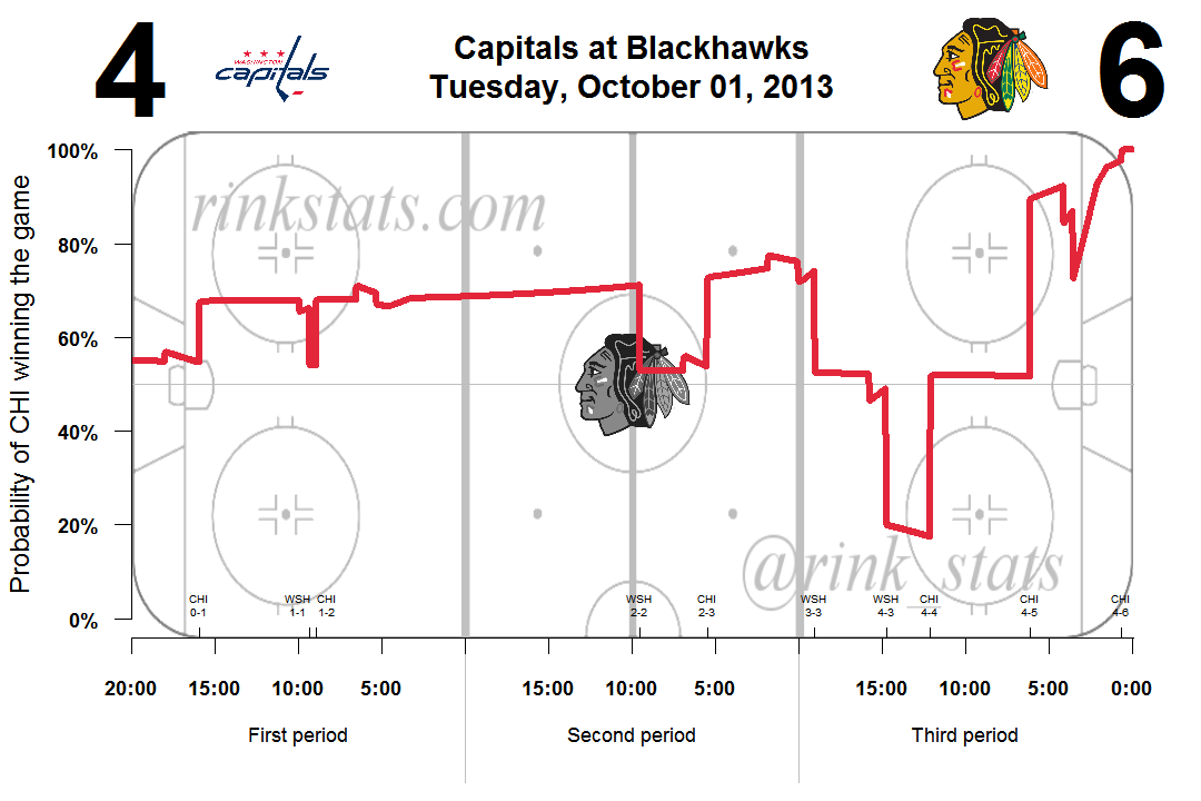
Above is the win probability graph from a Washington-Chicago game early this season. On the y-axis is the probability that the home team, Chicago, wins the game. On the x-axis is current time on the clock. Very astute hockey fans will notice that I’ve taken some liberty with the location of the blue lines. By making the neutral zone bigger, I’m able to make the blue lines correspond with the 1st and 2nd intermissions. Shh, don’t tell anyone.

Along the bottom of the graph is the time location of each goal scored in the game. This should give you a better idea of exactly what’s going on in the probability curve. You’ll notice that goals tend to correspond with the biggest swings in win probabilities.

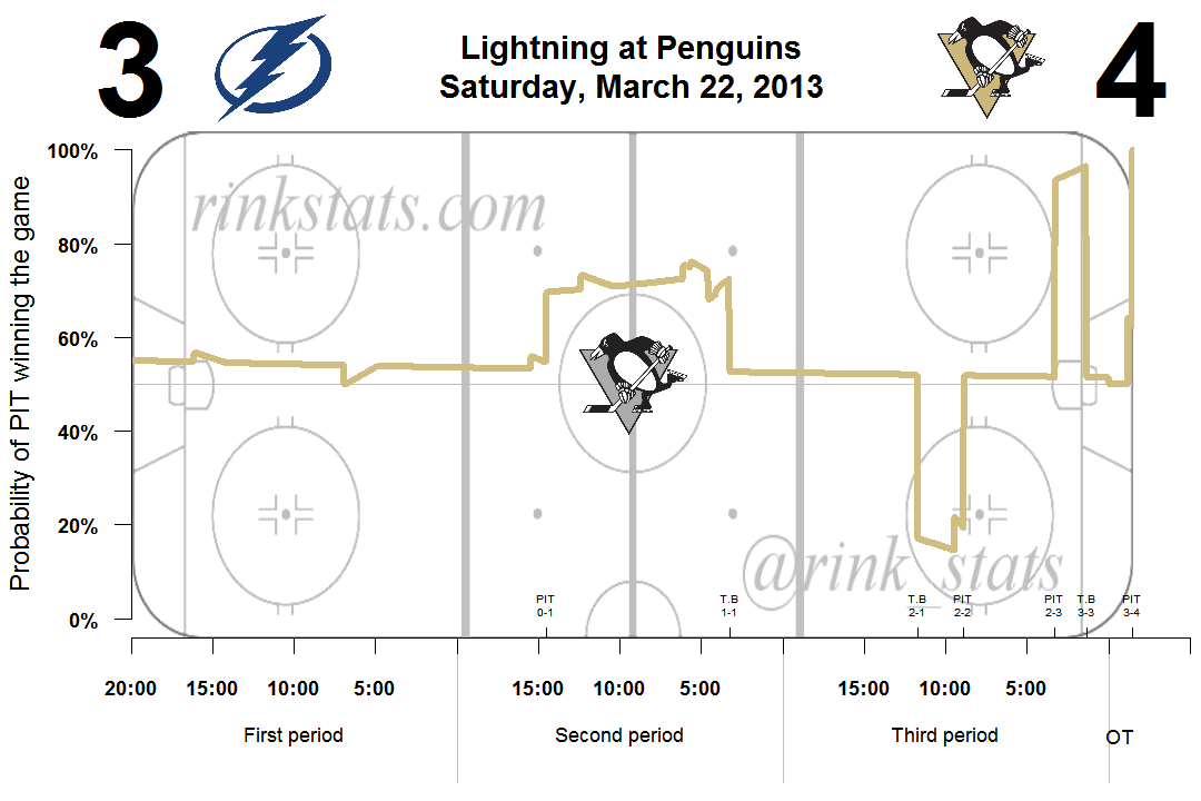
There’s also smaller peaks and valleys long the curve. These correspond with penalties which created power-play opportunities. You’ll notice in the graph above (which was featured in The Pensblog’s recap for this game), that Pittsburgh’s first goal of the game was scored when they were in the middle of one of these small spikes. This means that the goal was a power play goal.

One common thing that people have noted about the graphs is that they seem relatively flat. Shouldn’t the probabilities be converging to 0 or 1 when a team is leading? The model has this property, although it’s constructed in a way that does a better job of representing reality.

Imagine a team is ahead 1-0 five minutes into the 1st period. We would expect their win probability to increase over the next 60 seconds. But we wouldn’t expect it to increase nearly as much as it would in the time between 2 minutes and 1 minute remaining in the 3rd period.

You can see an example of this property in the TB/PIT graph. Pittsburgh is ahead by 1 goal for about 10 minutes in the second period and their win probability increases a few percentage points. The slope is relatively flat. But look at the third period. Between Pittsburgh and Tampa’s third goals, the Penguins win probabilities increase by a few percentage points also, except this time it occurs in just 90 seconds.

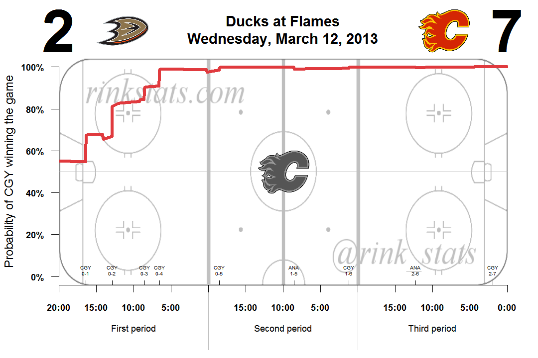
The model has other intuitive properties. A team that scores a goal in a tied game will have a much larger spike in its chance of winning the game than a team that scores when they’re already ahead by several goals. This can be seen in the graph above, which shows the probability curve for a blowout game.

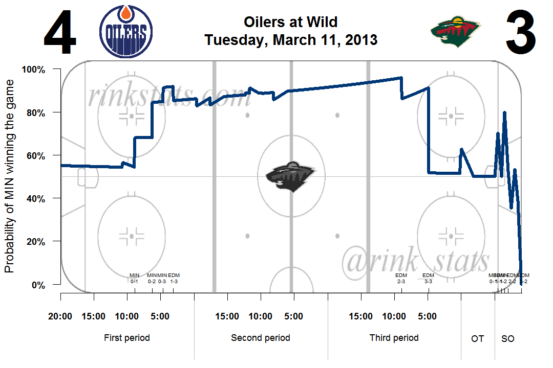
I’ve also built shootouts into the graphs. You’ll notice in the graph above that the win probabilities do a lot more jumping around during the shootout, depending on whether each shooter did or did not score. This is because the results of each shot attempt tremendously impacts a team’s chance of winning the shootout. If the first shooter misses, their team’s win probability drops dramatically because they now only have two more attempts (to their opponent’s 3). If the first shooter scores, their team’s win probability spikes.

I’m still trying to figure out a good way to represent shootout goals, since I have the obvious problem of text overlapping itself. Any ideas are welcome.

The stats behind the model

The basic guts of the model is a smoothed version of the conditional probability of the home team winning the game, given the current score and time remaining in the game. To get these probabilities in regulation time, I took 7 seasons of data (~8000 games), determined the score at all 3600 seconds (60 minutes x 60 seconds) and calculated the percentage of time the home team won the game at each of the different score differentials. The graph of these empirical results is below. The title of the graph indicates that these probabilities are smoothed. I used a very low information Bayesian beta prior to get rid of some of the noise resulting from fewer than a couple datapoints (particularly for rare games with big goal differentials very early in the games).

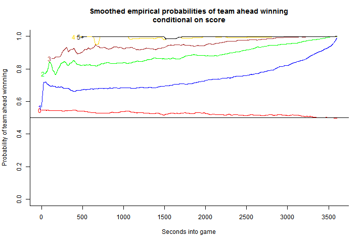
One note about the graph, and the model, is that I pool together all situations in which a team is head or behind by 5 or more points. Also, you’ll notice that in tied games the probability of the home team winning is greater than 50%. This represents the empirical estimate of home-ice advantage. For all non-tied scores, I take home-ice advantage out of the calculus by taking the absolute value of the score difference and averaging based on the probability that the team ahead wins the game.

My next step was to get rid of some of the jitteryness of the empirical graphs. I assume that the small bumps in the lines in the graph above are just statistical noise due to differential sample sizes and variance in the underlying data generation process.

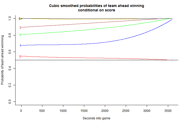
In order to smooth these curves out, I estimate five simple OLS models where the outcomes variable in each is the is the win probability given the score differential and the explanatory variables are time (in seconds), time squared, and time cubed. I also restrict the model such that the curves for each non-zero score differential must converge to 1 as time reaches 3600 seconds.

I use the estimated coefficients to get a smoothed version of the first graph. Note: Because I used OLS, in a couple situations the model estimates win probabilities of higher than 100%. In these cases I set the probability of winning to be a value arbitrarily close to 100% (0.9999). The results from the regression smoothed win probabilities is below.

The next step in building the model was to incorporate penalty information. The datawork behind this was no easy task. I’ve been trying for the better part of a year to get the number of seconds remaining on penalties from the play-by-play. The data on the NHL’s website doesn’t explicitly have this, so I had to learn the intricacies of the NHL rulebook, turn the rules into code, and put in about a million exceptions for very bizarre game situations or errors in the HTML for the original play-by-play on nhl.com.

Once I had the number of seconds remaining at each strength for every second in each game (5-4, 4-4, 4-5, 3-4, etc.) I calculated the powerplay and shorthanded scoring rates. Then, for times in the game which were not played at full strength, I use the law of total probability to calculate the win probability of the home team if they’re on a power play:

Of course this formula isn’t exactly an equivalency. I’ve left out the possibility of multiple sort-handed goals, as well as multiple power play goals (on a major penalty). But the probabilities of multiple PPG or SHGs occurring on the same penalty are so small that assuming them away has virtually no effect on the model.

So far, this gives us the win probabilities for the 1st through 3rd periods. For overtimes, I take a slightly different approach. Home ice-advantage is virtually nil in overtimes, so when the teams are at even strength, I assume the probability of either team winning is 50%. For home powerplay situations I’m able to reduce the formula above slightly:

This formula implies that powerplays in overtime will create bigger spikes and troughs in the win probability curves, since the probability of winning reduces to the probability of scoring once in overtime.

The last thing I put into the model is shootouts. For the first 3 rounds I use 7 seasons of data to get the probability of a team winning, conditional on which shooter (1 through 6) is up and what the score differential is. I collapse together rounds 4+ and condition on whether it’s the first or second shooter of the round and (for the second shooter) whether or not the first scored.